Section 03 · The Bench E-12
From tube to number
Thermal desorption, separation, detection, integration: four steps, each with its own way of being wrong.
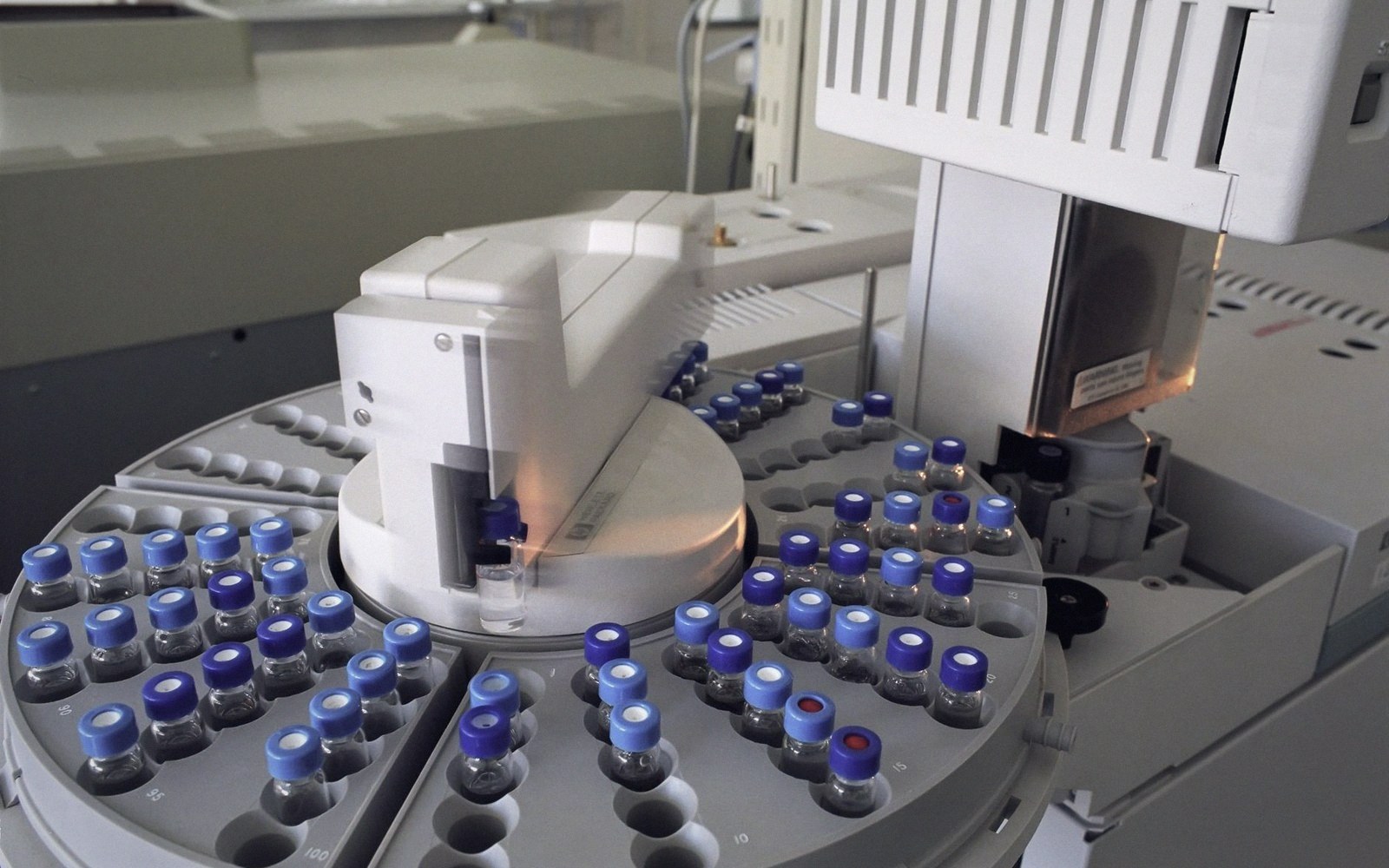
The heat that starts the clock
A pumped sorbent tube leaves the field sealed, labelled, cold-stored. In the laboratory, it goes onto a thermal desorption (TD) unit — a device that heats the tube to a temperature high enough to drive everything trapped in the sorbent bed back into the gas phase. That gas is swept by a carrier gas, typically helium or nitrogen, onto a small focusing trap cooled to sub-ambient temperature. The trap concentrates the analytes into a tight band; then it too is heated rapidly, and the analytes are injected — all at once, as a narrow pulse — onto the head of a gas chromatography (GC) column.
The first failure mode lives here. Desorption temperature and hold-time must be long enough to transfer everything off the sorbent, but if an analyte's boiling point is close to the desorption temperature, or if the cold trap is not cold enough, part of the analyte misses the column entirely. A compound that desorbs incompletely appears to be present at lower concentration than it actually is — a negative bias that no downstream step can correct. This is the territory of recovery: the fraction of what went in that actually came back out.

Along the column
The GC column — a capillary, typically 30 to 60 metres of fused silica with a coated inner wall — separates compounds by the interplay between their affinity for the coating and their tendency to remain in the carrier-gas phase. Compounds that interact more strongly with the stationary phase move more slowly; they reach the detector later. Each compound produces a peak in time, and retention time — the moment of that peak — is the primary basis for identification.
The second failure mode is co-elution: two compounds with similar properties reaching the detector at the same moment, their signals merged into one. A single peak is attributed to one compound, the other's contribution is invisible, and the quantification of both is wrong. Column choice and temperature programme are the defences, and laboratories validate them. But complex real-world air samples can still produce interferences that a clean analytical standard never revealed.
What the detector sees
Most volatile-organic work uses a flame ionisation detector (FID) or a mass spectrometer (MS). The FID responds to carbon bonds — robust, linear over several orders of magnitude, but non-specific: it cannot distinguish which compound generated the signal. The MS breaks molecules into characteristic fragment ions and compares the resulting pattern against a library; it adds a second dimension of identification. Neither detector is universal: the FID is blind to inorganic compounds; the MS response factor varies with ionisation efficiency, and some compounds share fragment-ion patterns closely enough to require a reference standard for confident identification.
The third failure mode is matrix interference — something in the sample that shifts detector response for the compound of interest. A dirty column bleed, a co-eluting compound not resolved by the separation, a carrier-gas impurity: any of these can raise or suppress the signal. Calibration standards run in the same matrix as the sample are the defence; calibration standards run in clean solvent are not.
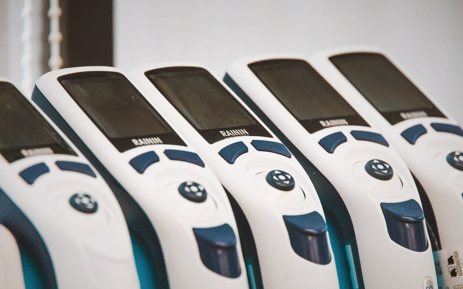
Where the operator draws the line
The detector signal is a trace — voltage against time — and at the end of the column run it is a landscape of peaks and valleys. Integration is the act of defining where each peak starts and stops and calculating the area under it. That area is then compared to the calibration curve to yield a concentration.
Integration is where human judgement re-enters a process that has been almost entirely automated until this moment. A peak riding on a rising baseline, a shoulder that may be two compounds or one asymmetric one, a small peak in a noisy region near the detection limit — each demands a decision. Software defaults do not always make the right one. A skilled analyst inspects every integration manually for any peak that will appear in the final report. The number at the end of the chain — the concentration written in the report — rests directly on where that line was drawn.
Four steps, four vectors of error. None of them cancels the others.
Filed inSection 03 — The Bench